
How-to Guide
Part 5: A Witless Fool, Building an LLM From Scratch in Rust

February 16, 2026
We have spent four parts building a Large Language Model engine. We wrote the tokenizer, the self-attention mechanism, the feed-forward networks, and the training loop in Rust. Now we finally turn the key and take it for a ride.
When we wrote the example configurations for the Feste repository (named Tiny, Small, Medium, and GPT2), we hoped we were making reasonable choices. We had read papers, looked at existing architectures, and made educated guesses. Then we actually ran them, and what we thought would work didn't. What we thought would fail sometimes did better. The relationship between model capacity and training data turned out to be far less forgiving than we expected.
That confusion sent us down a path of systematic experimentation, isolating one variable at a time, and what we found contradicted a lot of our initial intuitions. Wider is not always better. More parameters do not guarantee better results. And validation loss can actively mislead you about model quality.
Here is how we went from those first confused results to a 9M parameter "Pocket Bard" that writes something that almost sounds like Shakespeare.
The Starting Point
We ran all four presets to completion. These were not optimized architectures for learning Shakespeare. They were our best guesses at the time. The results:
-
Tiny (64 embedding, 1 head, 2 layers, vocab 512) — 7 hours, 25,650 steps:
"To be, or not to been Holangnats an e-poorther livers" -
Small (128 embedding, 1 head, 3 layers, vocab 1,024) — 6 hours, 11,000 steps:
"To be, or not to behold with you wish, Pompey's friends" -
Medium (256 embedding, 4 heads, 4 layers, vocab 1,536) — 19 hours, 18,600 steps:
"To be, or not to behind! Are and modestroging rebellious chies" -
GPT2 (768 embedding, 12 heads, 12 layers, vocab 8,192) — 5.7 days, 37,300 steps:
"To be, or not to bees! You! CAL. Pead my master; made it shall I wee"
At first glance: gibberish. But the goal here was never memorization. A model that perfectly recites Shakespeare is just a very expensive lookup table. What we want is generalization: a model that has learned the patterns of Shakespeare's writing well enough to produce new text that sounds like it belongs. Every experiment that follows is chasing generalization, not recall.
Look at the results through that lens. The Tiny model produced nonsense words like "Holangnats." The GPT2 model, despite being orders of magnitude larger, gave us "bees" and "wee." We initially thought GPT2 was a disaster: 5.7 days of training for that? Yes, it sounds like juvenile potty humor, and that is actually kind of funny. Shakespeare himself was not above a good fart joke. But more importantly, "CAL" is a learned token from the character name CALPURNIA. The model picked up dialogue structure. And Small finished before Tiny (6 hours vs 7 hours) despite being slower per step, because it hit its validation plateau faster and early stopping kicked in. The "bigger" model learned what it could from its limited vocabulary sooner, then stalled. None of these presets were carefully tuned architectures. They were educated guesses.
This led to many weeks of laptop fans spinning up noisily, trying to improve upon those guesses.
The Experimental Setup
Before diving into results, a quick note on methodology. Each experiment isolates a single variable while holding others constant. We measure success primarily through perplexity, which you'll recall from Part 4 is the exponential of the loss. Stated more simply, a perplexity of 100 means the model is as uncertain as choosing randomly from 100 equally likely options. Lower is better.
A critical caveat: perplexity is only comparable across experiments using the same tokenizer. A smaller vocabulary makes perplexity artificially lower because the model is choosing from fewer options. We standardized on 8,192 tokens for all experiments so that perplexities are directly comparable.
We also watch the generated text. Numbers tell you the model is learning; samples tell you what it's learning. A model can have decent perplexity while producing grammatical nonsense, or struggle with perplexity while capturing something real about the style.
All experiments use the complete works of Shakespeare from Project Gutenberg: roughly 5.5 million characters tokenized into about 900K tokens with our BPE (Byte Pair Encoding) tokenizer from Part 1. We chose Shakespeare deliberately. The complete works are in the public domain, which means anyone can download the same dataset and reproduce our experiments exactly, and we sidestep the question of whether a model's outputs constitute reproduction of copyrighted material. Finally, neural network training is inherently stochastic: identical configurations produce slightly different samples at each step, though final perplexities tend to converge.
How Many Words Does a Model Need?
The GPT2 results in particular nagged at us. Its perplexity was higher than the smaller models, yet its output was clearly better. What did perplexity actually mean when comparing models with different vocabulary sizes? We spent several days in late November running tests based on a tiny architecture (64 embedding, 2 layers) with different vocabulary sizes to find out:
| Vocab Size | PPL | Sample Output |
|---|---|---|
| 512 | 35.2 | "To be, or not to beANnox. on�]eare �seru�ke Fir." |
| 2048 | 282.5 | "To be, or not to bething; should hath much re, nowpuble PARD." |
| 8192 | 119.3 | "To be, or not to befit. But I say thee at the dangerousing life when" |
| 16384 | 120.1 | "To be, or not to beguilts, that of poor every man to mine." |
The vocab-512 model has a deceptively low perplexity (35.2!) but produces garbage characters (�). It literally cannot represent the full character set. The vocab-2048 model avoids garbage but generates incoherent fragments. By 8,192 tokens we get coherent, Shakespeare-like output, and beyond that point compression gains flatten out.
To understand why, look at what each vocabulary actually contains:
- Vocab 512 sample tokens:
"thou"," this ","your ","have ",", and " - Vocab 8192 sample tokens:
"O, for the love of laughter","I have sworn thee fair","Farewell, young lord"
Both vocabularies use BPE, which starts with 256 single-byte tokens and iteratively merges the most frequent pairs. Vocab 512 allows 256 merges, enough to form common words like "thou" and "the." Vocab 8192 allows 7,936 merges, building longer and longer token chains. But by merge 7000+, BPE has exhausted the frequent pairs and starts merging combinations that appear only once or twice. Our token "I have sworn thee fair" was created at merge 7,178, and that exact phrase only appears in a single sonnet. The components were common; the final assembly was just mopping up. Beyond 8,192 tokens, we are creating vocabulary entries for phrases that barely exist. We settled on 8,192 as our standard: enough merges to capture Shakespeare's recurring patterns, few enough that training stays efficient, and a clean power of two.
Wide and Shallow vs. Narrow and Deep
Our first assumption was simple: bigger is better. We had two configurations ready to test, both using vocab 8,192 and 1,024-token context. The Medium model was wide and shallow: 256 embedding dimensions, 4 transformer layers, 4 attention heads. The Small model was narrow and deep: 128 embedding dimensions, 6 layers, 1 head. Medium had roughly double the parameter count. Surely it would win.
It did not.
We ran both models on the same data with the same hyperparameters, training until validation loss plateaued. Medium reached a perplexity of 220. Small hit 192. The smaller model, with half the parameters, learned better (Figure 1).
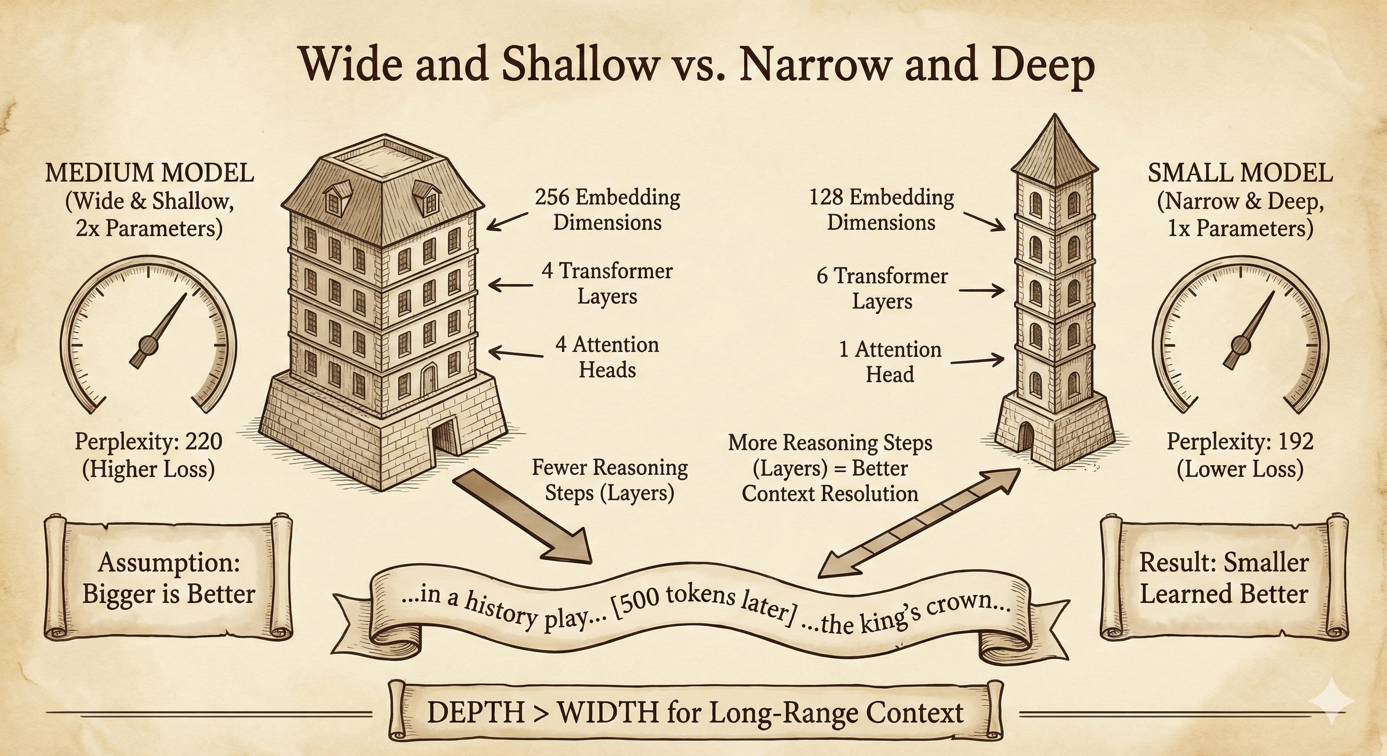
This result confused us until we thought about what language modeling actually requires. Consider the phrase "the king's crown" appearing 500 tokens after we established we're in a history play. Resolving that reference, understanding that "crown" here means royal authority rather than dental work or tree tops, requires the model to maintain context across many processing steps. Each transformer layer is a reasoning step, an opportunity to refine the representation. Width gives you more memory slots to store information. Depth gives you more opportunities to process it.
Shakespeare is deeply hierarchical. Meaning flows from words to phrases to sentences to scenes to acts. A wide shallow model can memorize patterns but struggles to compose them. A narrow deep model can build up understanding layer by layer, even with less raw capacity.
For our tiny models on this dataset, depth won. Whether that holds at different scales or on different data is another question.
Cyclops vs. Spider
Next we tested attention heads. The attention mechanism lets each token look at other tokens in the sequence to gather context. We wanted to understand a specific trade-off: is it better to have one attention head with high-resolution vision, or many heads with lower resolution each?
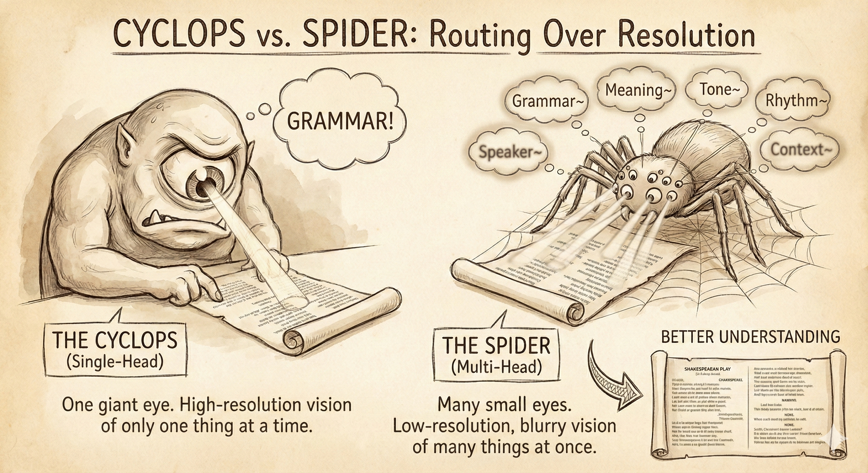
We took a tiny model (64 embedding dimensions, 2 layers, vocab 8,192, 64-token context) and compared two configurations with identical parameter counts. The single-head model (we called it "Cyclops") got the full 64 dimensions of resolution in one attention head. The eight-head model ("Spider") split that same capacity across 8 heads, giving each head only 8 dimensions to work with.
Our intuition said Cyclops should win. Each Spider head has such low resolution (8 dimensions) that we thought it would be too blurry to see anything useful. One clear view should beat eight fuzzy ones (Figure 2).
Again, we were wrong.
The 8-head model crushed the single-head model. Same parameter count, dramatically better results.
The problem with Cyclops is that when processing a word, it must simultaneously track grammar (what part of speech came before?), semantics (what topic are we discussing?), and long-range dependencies (who is the current speaker?). With one attention head, it can only look at one place in the sequence per layer. It has to choose: track the previous word for grammar, or track the speaker tag for dialogue formatting. It cannot do both at once.
The Spider model can look at 8 different places simultaneously. Each head might have blurry 8-dimensional vision, but together they cover far more ground. One head tracks the previous word. Another tracks the speaker tag. A third watches for repeated phrases. The combination wins decisively.
In our tests, routing beat resolution. The ability to attend to multiple positions mattered more than the clarity of any single attention pattern. This finding held even when we pushed the per-head dimensions quite low.
Working Memory
We tested context length next. The context window determines how many previous tokens the model can see when predicting the next one. We expected longer context would help the model write longer coherent passages. That turned out to be true, but not just for the reason we expected.
We used our Medium model (vocab 8,192, 256 embedding dimensions, 4 layers, 4 heads) and compared a shorter 128-token context against a longer 1024-token context.
The long-context model was significantly better by perplexity (a 40% improvement). But the surprise was that it wrote better short passages too. The initial assumption was that context length would only matter for generating long text, but it generally matters for training stability.
During training, we feed the model sequences and ask it to predict the next token at each position. With a 128-token context, the model sees tiny snippets. A speech might be cut off mid-sentence. The model has to guess what comes next with almost no information about where it is in the play. These impoverished predictions produce noisy gradients. The model thrashes around during optimization (Figure 3).
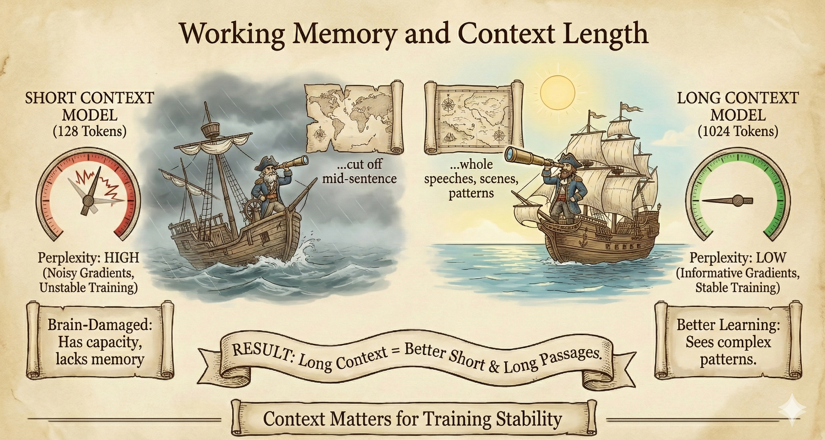
With a 1024-token context, the model sees whole speeches, sometimes whole scenes. It can learn that ROMEO's lines follow a certain pattern, that scene transitions have particular markers, that act endings differ from mid-act dialogue. The gradients are more informative. Training stabilizes.
A model with high capacity but short context is effectively working with blinders on. It has the processing power to understand complex patterns but lacks the working memory to see them during training.
Data Starvation Bug
With these results in hand, we built bigger models. The "Golden Ratio" configuration (128 embedding dimensions, 8 layers, 2 heads) had 3.7 million parameters. The "Modern" (192 embedding dimensions, 6 layers, 3 heads) pushed to 5.8 million. These larger models should have dominated our tiny 1.2 million parameter baseline.
They performed terribly. Golden Ratio hit a perplexity of 485 while the 1.2M model sat at 106.
We spent two days debugging. We checked the architecture, the training loop, and the hyperparameters. We even rewrote the backward pass, convinced we had a gradient bug somewhere.
Then we found it. A hardcoded limit in our data loader was restricting training to 500KB of text, about 9% of the Shakespeare corpus. The larger models had memorized that 9% perfectly. Training loss went to nearly zero while validation loss exploded. We hadn't created language models. They were lookup tables (Figure 4).
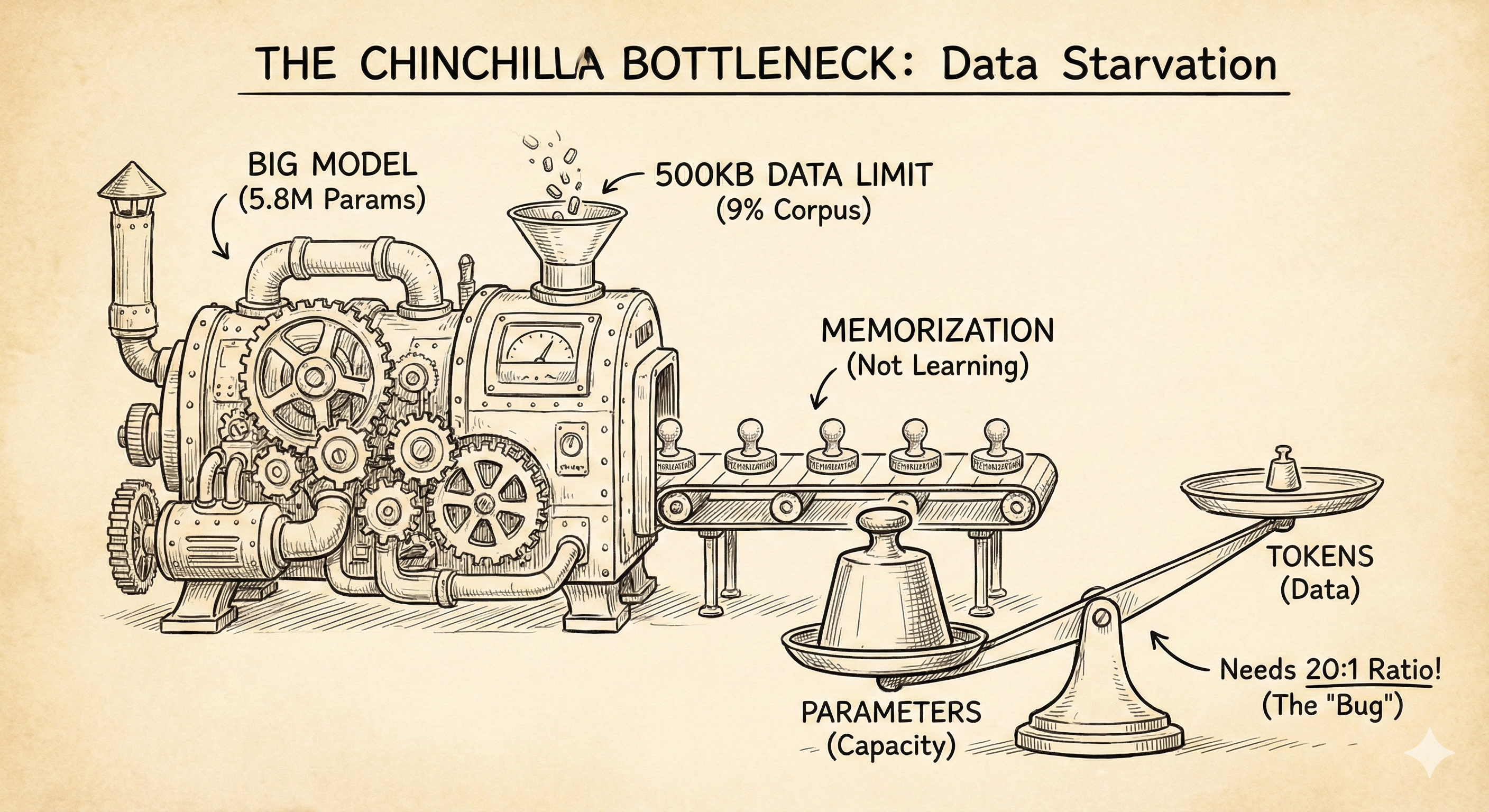
This was an accidental demonstration of the Chinchilla scaling laws: you cannot scale up the model without scaling up the data. The relationship between model parameters and training tokens is roughly 20:1 for compute-optimal training. Our 3.7M parameter model needed about 74 million tokens. We gave it around 80,000. After fixing the data loader to use the full corpus, the larger models started behaving sensibly. Architecture turned out to be irrelevant until we fixed the data problem.
Pocket Bard
We applied everything we had learned: deep over wide, many heads, long context, full dataset. The result was our best from-scratch configuration: Pocket Bard.
The architecture had about 9 million parameters: vocab 8,192, 256 embedding dimensions, 6 transformer layers, 12 attention heads (21 dimensions each), and a 448-token context window.
We trained until validation loss plateaued and achieved a final perplexity of 92.
Here is what the model learned to do:
-
Step 0:
"To be, or not to be; had fit feeFlorion is tendantat all odhownone" -
Step 8600:
"To be, or not to beLest I am y his eyes know the lipso is. [Exit.]" -
Step 17000:
"To be, or not to be—in handard to our t. KING HENRY. O, Protil-belli" -
Step 42000:
"To be, or not to befall; yet so love I love the again. MARINA. Then"
By step 8600, stage directions emerge: [Exit.] in proper bracket notation. By step 17000, the model produces KING HENRY, a real character from the history plays. And by step 42000, we see MARINA from Pericles, surrounded by surprisingly coherent phrasing: "yet so love I love." The model learned to produce actual Shakespeare characters, not just plausible-sounding invented names.
The model has absorbed something real about how Shakespeare sounds. Not just individual words, but the structure of a play: character names on their own lines, stage directions in brackets, the rhythm of dialogue.
But you don't have to look too deeply to spot the cracks. We tested with various prompts at temperature 0.8. Temperature is a scaling factor applied to the model's raw output scores before they become probabilities. At temperature 0, the model always picks the single most likely next token, which is deterministic and tends to get stuck in loops. At temperature 1.0, it samples directly from the learned distribution, which can get wild. Too low and our model looped endlessly on character names, stuck repeating "GLOUCESTER. GLOUCESTER. GLOUCESTER." Too high and it dissolved into incoherence. At 0.8, we found the sweet spot where the model takes risks without losing coherence.
- Short prompt ("To be"): The model panics. With minimal context, it cannot lock onto a genre or character. Outputs become collisions of half-remembered patterns, character names mashed together, words invented from plausible-sounding fragments.
- Long prompt (a full speech): The model settles. Given enough context to establish genre and tone, it produces coherent continuations. Tragedies stay tragic. Histories maintain their formal register. Comedies remain lighter.
- Semantic probes: The model hallucinates. It generates words like "disoberontful" and "behalvillain" that follow English morphological patterns but mean nothing. It knows how to construct words but not what things are.
This is the fundamental limitation at 9 million parameters. The model has learned syntax, format, and style, but it has not learned semantics. It can produce text that sounds like Shakespeare without understanding what the words mean. We have built something like a person singing along to a song in a language they don't speak. The rhythm is right. The sounds are plausible. But the words are invented, and meaning is entirely absent.
At this point, we concluded that a perplexity of 92 represents something like a floor for this architecture on this data. The remaining uncertainty is not noise the model could learn away with more training. It is genuine ambiguity (places where any of many next tokens are equally valid) plus the model's semantic blindness to word meaning.
Teaching English Before Teaching Shakespeare
We found ourselves with a model that could produce Shakespeare-flavored fragments, but perplexity had flatlined in the low 90s and no amount of hyperparameter fiddling would move it.
Not ready to give up, we wondered if we could fine-tune an existing model to achieve our goals. But that felt like cheating for an educational project about building transformers from scratch. We wanted to understand pre-training, not just benefit from someone else's. Besides, there were no obvious small models to use as a starting point for Shakespeare specifically.
Then we found TinyStories.
TinyStories came out of Microsoft Research in 2023. Ronen Eldan was reading bedtime stories to his daughter and started wondering: how did she learn language with such limited vocabulary? That question led to an experiment. The researchers generated millions of synthetic children's stories using GPT-3.5 and GPT-4, constrained to vocabulary a typical 3–4 year old would understand. Simple sentences, clear causality, basic narrative structure. "Tom liked to ride bikes. He played all day."
The results were impressive. Models with fewer than 10 million parameters, trained on TinyStories, could produce fluent and grammatically correct text. The same architectures trained on web text produced garbage. The dataset proved that small models could learn coherent English if the training data was appropriately scoped. TinyStories later influenced Microsoft's Phi series of small language models and became a standard benchmark for studying how language capabilities emerge at small scales.
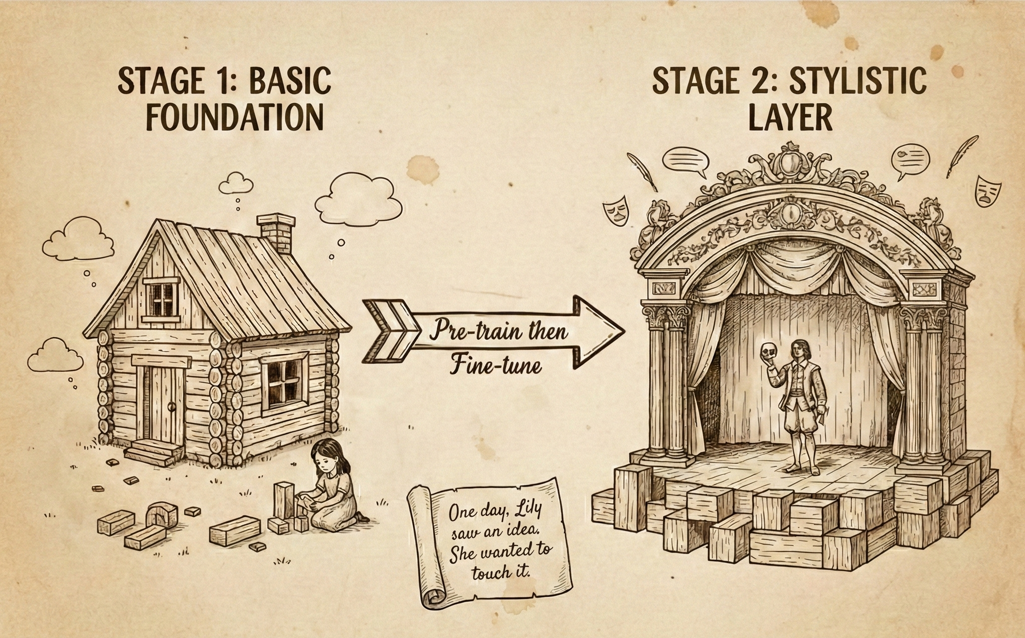
This gave us an idea. Our 9M parameter model was spending most of its capacity learning basic English (word boundaries, common phrases, grammar rules) while also trying to learn Shakespeare's style. What if we separated those tasks? Pre-train on TinyStories to learn English fundamentals, then fine-tune on Shakespeare to learn the style.
The TinyStories Base Model
We trained a new tokenizer on the combined TinyStories and Shakespeare text, keeping the same 8,192-token vocabulary size. This ensures the model can represent both datasets, though the token distributions differ. We then took our 9M parameter architecture and pre-trained it on TinyStories until validation loss plateaued.
The model learned clean English. Grammar was solid. Sentence structure was correct. Vocabulary was limited but used properly. One sample from the best checkpoint shows just how well:
Once upon a time... there lived a little girl named Lily.
One day, Lily saw an idea. She wanted to touch it.
"Lily saw an idea. She wanted to touch it." The model learned that you can "see" and "touch" things, and that "idea" fits grammatically in the same slot as "ball" or "bird." It does not know the difference between concrete and abstract. It just knows the grammar (Figure 5). That distinction will matter later.
Another example:
One day, Lily's mom told her about the big red ball in the sky.
As Lily was playing, she saw a boy named Bob.
Multiple characters, reported speech, scene-setting. The model picked up the full machinery of narrative, not just grammar but story structure. All of it learned from nothing but next-token predictions on children's stories.
Pre-training complete (TinyStories):
- Prompt:
"The King said" - Output:
"The King said, 'Hi Kitty!' Sue said, 'Yes! I like my ice cream!'..." - Perplexity: 9.68
Responding to this prompt, the model saw "King" and immediately defaulted to its native language: cheerful children's stories. The grammar was perfect, and the content was appropriate for a three-year-old. The word "King" in TinyStories means a character in a fairy tale, not a monarch in a history play.
Fine-Tuning on Shakespeare
We loaded the TinyStories checkpoint and resumed training on the complete works. What followed was a tug-of-war between the two styles that taught us something important about validation metrics.
-
Step 0 (fresh from TinyStories):
- Sample:
"To be, or not to be. My lord, tonight hath another strong wolf a whil" - Perplexity: 24.66
- Sample:
Before a single step of Shakespeare training, this model already has a lower perplexity (24.66) than our best from-scratch model achieved after weeks of training (92). English fundamentals like grammar, word boundaries, and sentence structure transfer directly, even across radically different domains.
But look at the sample. "Hath"? The model has never seen Shakespeare, and it turns out it's not actually producing Early Modern English. Instead, the prompt is completely out of distribution for a model trained on children's stories. The model has no basis for predicting what comes next in this context, so instead of strongly favoring a few likely tokens, it spreads probability thinly across its entire vocabulary. Temperature-based sampling can then land on almost anything, including "hath."
We ran this checkpoint multiple times and got wildly different outputs each time. The model is rolling dice over its vocabulary. What is real here is "strong wolf," which is pure children's story vocabulary, and the grammatical scaffolding holding the sentence together. The model has English fundamentals. Now it is seeing Shakespeare for the first time.
-
Step 1200 (best perplexity):
- Sample:
"To be, or not to be.\n\nBASSANIO. Hearreste, my lord,—" - Perplexity: 22.44
- Sample:
By step 1200, the model has picked up character names and play formatting. This is the best perplexity we achieved. By the validation metric, we should stop here.
We kept training, even though the perplexity started climbing.
-
Step 35000:
- Sample:
"To be, or not to belie but to perish [_Kneeling_.] To wait, was loath" - Perplexity: 27.36
- Sample:
The model has learned physical stage directions in proper notation. The phrasing is dense, compressed, theatrical. The validation loss keeps climbing.
We pushed to 40,000 steps, deliberately inducing what the machine learning literature calls "catastrophic forgetting." The model was losing its ability to perform on the original TinyStories distribution. We wanted to see what happened when it fully committed to Shakespeare.
-
Step 40000 (final):
- Sample:
"To be, or not to be rose from me Because another.\nIMOGEN. No matter m" - Perplexity: 27.96
- Sample:
The validation metric says this is worse than step 1200. The samples say otherwise.
What This Taught Us
The jump from a TinyStories perplexity of 9 to a Shakespeare perplexity of 22 is straightforward. Shakespeare presents a harder prediction problem. A children's story sentence might continue with "said" or "went." A Shakespeare sentence could continue with "quoth," "spake," or "didst go." More valid continuations means more uncertainty, and perplexity measures uncertainty.
The climb from 22 to 27 is a different phenomenon. As the model committed to Shakespeare's distribution, it abandoned the safe generic English predictions that had kept perplexity low. Choosing "quoth" over "said" is stylistically correct but statistically riskier. The model spreads probability across archaic alternatives that the validation set may not reward at any given position. The metric saw growing uncertainty. The samples showed growing competence.
We had to train past the mathematical optimum. The best checkpoint by the numbers (step 1200) was not the best checkpoint by the ear (step 40000+). The only way to know when to stop was to watch the generated samples. When the model stopped producing any trace of TinyStories, when every output was unmistakably theatrical, we stopped.
The Full Picture
We have been showing you curated samples throughout this section. The Shakespeare-only model from "Pocket Bard" could produce real character names and coherent fragments when conditions were right, particularly with longer prompts and favorable temperature settings. But pull back and look at a broad sample of outputs, and the picture changes. We took both models, the transfer learning model and the Shakespeare-only model from "Pocket Bard", and generated a batch of samples under identical conditions. Same architecture, same 9 million parameters, same vocabulary. The only difference was the starting point.
The transfer learning model produced real character names (BASSANIO, MACBETH, OLIVIA), stage directions in proper notation, and phrases that scan as English. Not all of it makes sense. But the building blocks are right.
The Shakespeare-only model, the one whose cherry-picked samples we showed you earlier, produced BUTSA, DGRIVERS, and HESTANS. It produced "beesponounce arrow" and "bmbLur these fwith ganed auy." It's not generating English, it's generating something that occasionally bumps into English on its way somewhere else (Figure 6).
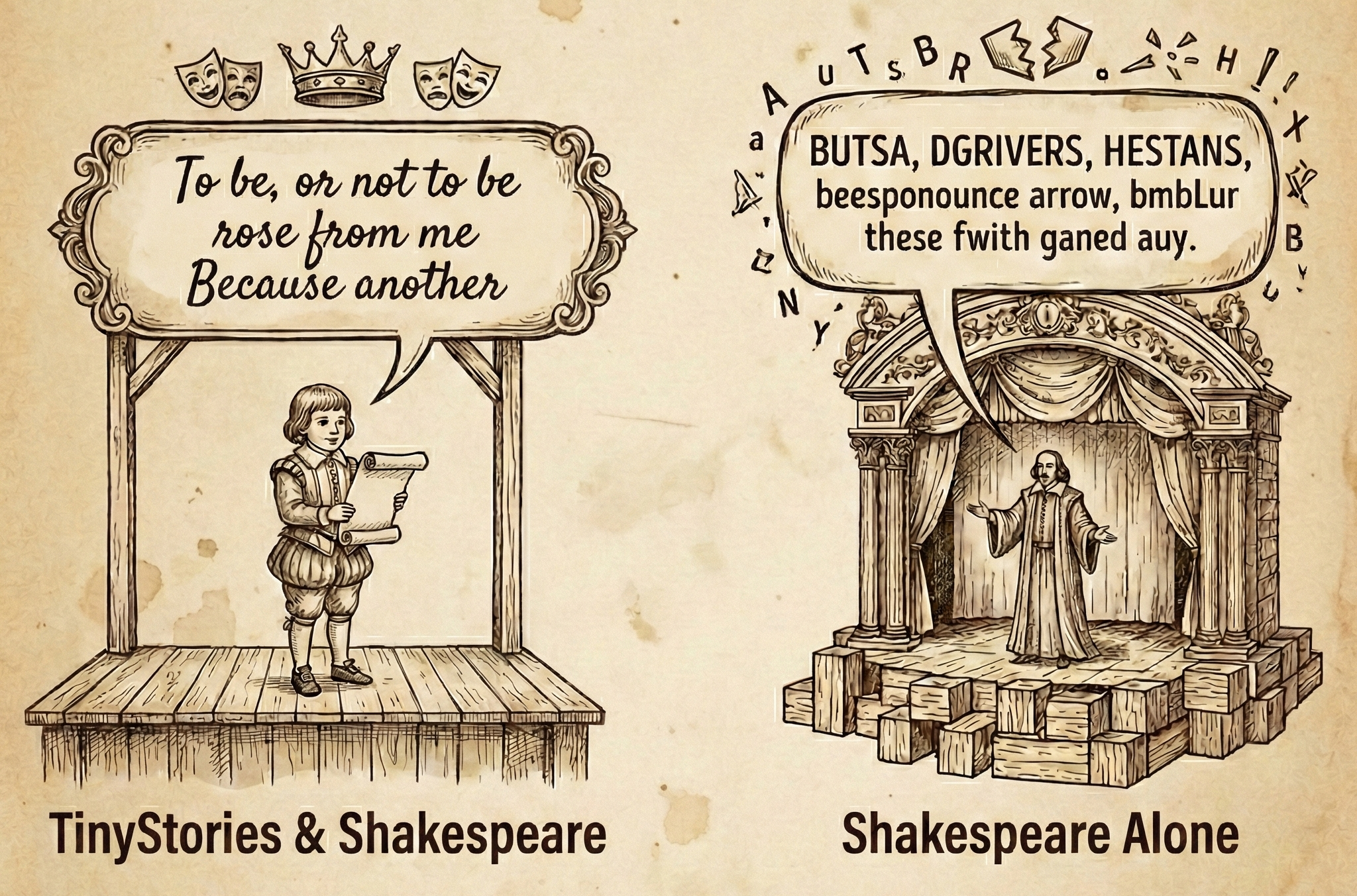
One model knows how English works and is learning Shakespeare's particular dialect of it. The other is trying to learn both simultaneously from 900,000 tokens, and that is not enough.
This is what transfer learning actually buys you at small scale. The TinyStories pre-training taught the model word boundaries, capitalization patterns, sentence structure, and how dialogue works. Fine-tuning on Shakespeare then only has to teach vocabulary and style, which is a much smaller problem. Training from scratch has to learn all of it at once from a corpus two orders of magnitude too small for the parameter count. As we saw with the data bug earlier, the Chinchilla ratio says our 9M model wants 180 million tokens and Shakespeare gives us less than one million. Transfer learning allowed us to survive that gap.
What Worked
After weeks of experiments, here is what we took away. Remember however, we were training 9M parameter models on CPUs, so none of this is remotely frontier-scale advice.
- Go deep, not wide.
- Use many attention heads.
- Train with long context even for short outputs.
- Watch the samples, not just the loss.
All of these conclusions emerged from the experiments above, and many of them contradicted our initial assumptions.
If we were starting over, we would skip the vocabulary size experiments entirely and start at 8,192. We would not bother with wide-and-shallow architectures. We would begin with transfer learning from day one instead of spending weeks on from-scratch training that hit a wall at perplexity 92. And we would build a proper evaluation pipeline instead of eyeballing samples, because "sounds Shakespearean to me" is not reproducible science, even if it turned out to be more informative than the loss curves.
What We Built
We set out to understand how language models work by building one from scratch. No PyTorch, no TensorFlow, no external ML libraries: just Rust, a text editor, stubbornness, and a public domain corpus anyone can download. We wrote a BPE tokenizer that compresses Shakespeare into dense tokens. We implemented tensor operations that run efficiently on the CPU. We built the transformer architecture (attention, feed-forward networks, layer normalization, all of it) with explicit backward passes we derived by hand. We created a training loop with AdamW optimization, gradient clipping, learning rate scheduling, and checkpointing. And it works.
And now we have a model that writes like this:
Prompt:
"ROMEO:"ROMEO: this be true.
BENET. Come, come, it doth so.
ROMEO. I shall have it on you.
JULIET. No, no. Stay thou, that I met.
ROMEO. No, not for love.
JULIET. That of the sound when my love: I'll marry
I showed this to my wife, who minored in Shakespeare and who has heard rather a lot from me about what I've been working on. She read the output, paused, and begrudgingly admitted it kind of sort of has the rhythm. "But you know it's garbage, right? It's not really saying anything."
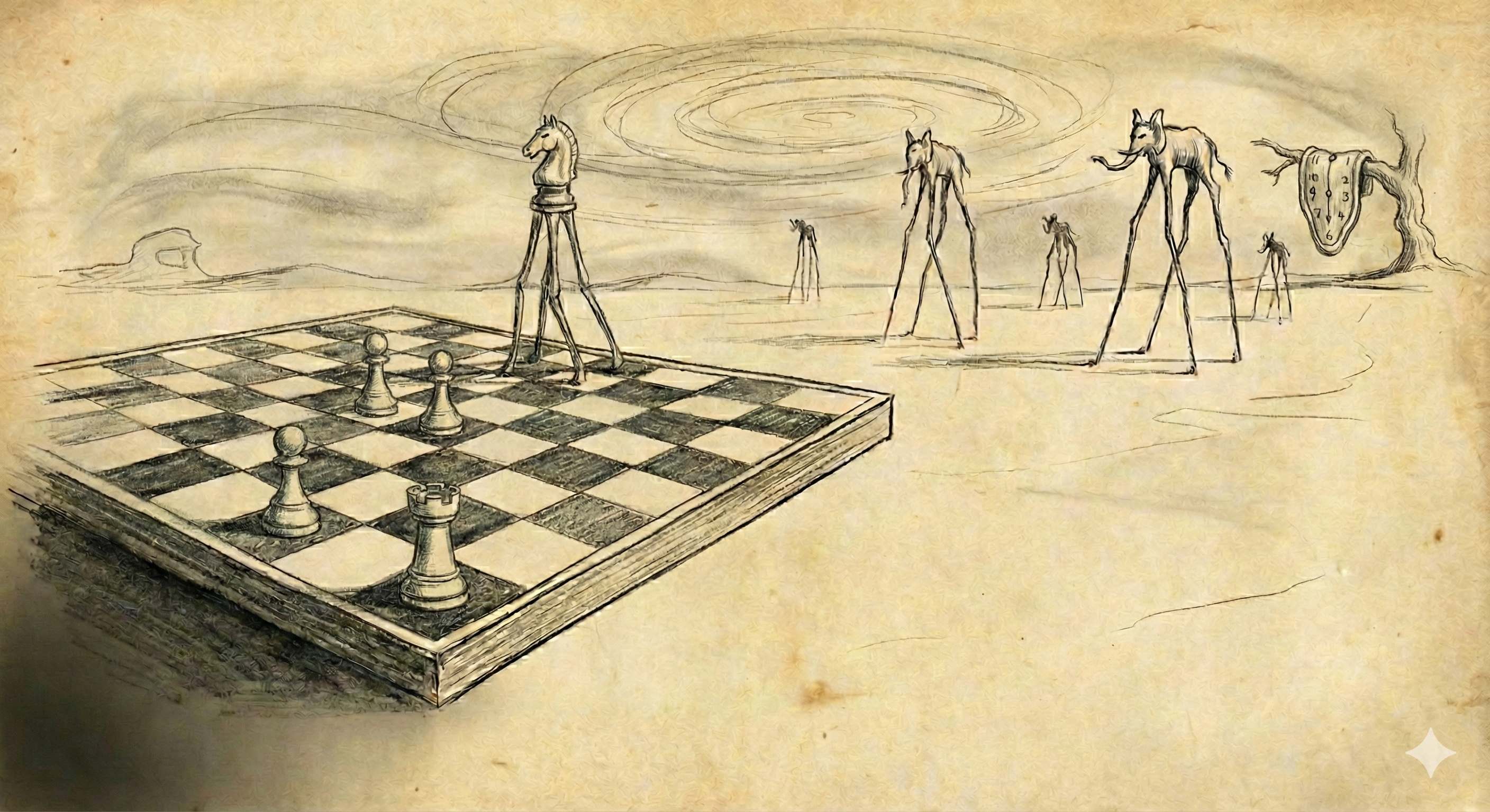
She then told me about an assignment during her studies where she had to paint an original work in the style of Dalí. It wasn't about reproducing or analyzing his paintings. She had to create something new that looked like it belonged in his catalog. She spent weeks on it and was proud of the result. The hard part, she said, was painting something that fit his style without actually copying or borrowing from what Dalí had already painted. And she's right that what she produced and what our model produces are fundamentally different things. She understood the work. She had opinions about what the imagery meant, why a melting clock lands and a random surrealist juxtaposition doesn't, how composition creates tension across a canvas. Originality within a style was hard for her. Meaning was the easy part (Figure 7).
For our model, it is exactly the reverse. Rhythm, formatting, character names, dialogue structure, iambic meter: all of that fell out of the statistics. What the model cannot do, what 9 million parameters trained on 900,000 tokens will never do, is understand what any of it means. It learned everything that can be learned by pattern matching. It learned nothing that requires comprehension.
That gap is the most important thing we discovered. Not a hard boundary on what statistical learning can do, because frontier models with billions of parameters trained on trillions of tokens clearly develop something that looks a lot like comprehension, but a clear picture of what it takes to get there and how far 9 million parameters on 900,000 tokens falls short. Our model and my wife approached the same problem from opposite ends. She wrestled with creating something original that still felt authentic to the artist's style. The model never had a chance at the meaning. Scale and data may eventually close the gap from the model's side. But at our toy scale, the boundary is vivid.
We started with random weights that produced noise: "feeFlorion is tendantat all odhownone." We ended with a model that produces grammatical Early Modern English with appropriate character names and theatrical cadence. The weights are no longer random. They encode something real about the structure of Shakespeare's writing, even if they encode nothing about its meaning.
That is what training does. It takes random noise and shapes it into patterns that capture statistical regularities in data. We saw word boundaries emerge, character names click into place, iambic rhythm appear from nothing. We also saw where it stopped, and now we understand why.
We did not build a frontier model. We built a toy. But it was fun to build and fun to play with, and we understand every piece of it. The complete code is available in the Feste repository. If you want to understand how transformers actually work, there is no substitute for watching gradients flow through one you built yourself.